How to Use VLOOKUP in Excel

You know the VLOOKUP syntax. =VLOOKUP(value, range, column, FALSE). You’ve memorized it. You’ve used it a hundred times. And it still breaks on you every other week.

That’s not a formula problem.

I watched a financial analyst spend four hours debugging a VLOOKUP formula yesterday. The formula was perfect. Her data was garbage. This happens every single day, and VLOOKUP is a fast and easy way to find information when the data is organized in columns, but that “when” is doing all the heavy lifting here. Most failures happen because the data structure was never lookup-ready in the first place.

The formula’s easy. You can Google it in 30 seconds. What kills you is the invisible stuff: spaces you can’t see, numbers that look like text, duplicates hiding in row 847. I’ve watched experienced analysts waste entire afternoons hunting for typos when the real problem was someone copy-pasted from a PDF six months ago.

Yeah, AI tools like Copilot can write VLOOKUP for you now. Excel Copilot now eliminates the need for complex formulas like VLOOKUP by allowing users to perform data lookups with plain English commands (Geeky Gadgets). But AI can’t fix your underlying data problems. It’ll just write a perfect formula that returns #N/A for every single row because your lookup values have trailing spaces.

Table of Contents

• The Diagnostic Skills Nobody Teaches

• How Excel Actually Thinks About Lookups

• Fix Your Data Before You Touch That Formula Bar

• Writing VLOOKUP Formulas (The Right Way)

• The Left-Side Thing Everyone Hates

• Exact vs. Approximate Match (Get This Wrong and You’re Screwed)

• Error Handling That Actually Works

• When VLOOKUP Becomes the Wrong Tool

• Building Formulas That Won’t Break Next Month

• Moving Beyond VLOOKUP Without Breaking Everything

Quick Version

Your data structure matters more than your formula. Fix the table before you write a single =VLOOKUP.

Always use FALSE for exact match unless you actually understand approximate matching (you probably don’t).

VLOOKUP breaks when you scale. Know when to switch to INDEX MATCH or XLOOKUP before you’re drowning in maintenance.

The left-side limitation isn’t a bug. It’s telling you to reorganize your data.

Every VLOOKUP needs error handling. Every single one.

The Diagnostic Skills Nobody Teaches

Think about the last time a VLOOKUP formula failed. Did you immediately check for formatting inconsistencies? Did you verify that your lookup column was positioned correctly? Or did you spend twenty minutes tweaking the formula syntax, hoping a different arrangement of parentheses would magically fix a data structure problem?

The formula itself is the easy part. You can memorize the syntax in five minutes.

What takes years to develop is the ability to look at your data and immediately spot why a lookup will fail. I’ve seen countless professionals struggle with VLOOKUP for months, convinced they’re missing some secret formula trick. They’re not. Their data has leading spaces, mixed formatting, or duplicate values that guarantee failure regardless of how perfectly they construct their formula.

Here’s what actually matters: your data setup. Get that wrong and no formula will save you.

Your VLOOKUP competency isn’t about memorizing parameters. It’s about developing the diagnostic skills to identify why your data isn’t lookup-ready and fixing those issues first. This is the part that separates people who use VLOOKUP successfully from those who fight with it constantly.

How Excel Actually Thinks About Lookups

VLOOKUP operates on specific logic that most users never explicitly learn. You’re telling Excel: “Find this value in the first column of this range, move across to a specific column number, and return whatever’s there.”

That sentence contains three critical decision points where things go wrong.

Excel starts at the top of your specified range’s first column and works downward, comparing each cell to your lookup value. The moment it finds a match (or determines one doesn’t exist), it stops searching and moves horizontally to your specified column. This sequential search pattern explains why VLOOKUP slows down with massive datasets and why the order of your data matters in approximate match mode.

Understanding this mechanical process helps you diagnose why you’re getting unexpected results. If you’re pulling the wrong data, Excel found a different match than you expected. Duplicate lookup values are the usual culprit. If you’re getting an error, Excel never found a match at all, which points to formatting inconsistencies or data entry problems.

Consider a customer database where you’re looking up customer ID “C-1045” to retrieve their email address. Excel starts at the top of your customer ID column and compares each cell: “C-1001” (no match, continue), “C-1023” (no match, continue), “C-1045” (match found, stop searching). It then moves right to your specified column and returns the email address.

But if you have duplicate entries (say “C-1045” appears in row 15 and again in row 47 with different email addresses), Excel will always return the email from row 15 because that’s where it stopped searching. The row 47 data is invisible to your formula. This is why duplicate lookup values cause silent errors that are extraordinarily difficult to catch.

The Three Questions Excel Asks

Every VLOOKUP execution involves Excel asking three questions:

Does this lookup value exist in the first column?

Which column should I return data from?

Should I find an exact match or the closest match?

Your answers to these questions (expressed through your formula parameters) determine everything. Most errors trace back to misunderstanding what you’re telling Excel to do.

The first question seems straightforward until you realize Excel’s definition of “exist” is more rigid than yours. You see “100” and “100” as the same. Excel sees a number and a text string as completely different values.

Decision Point	What Excel Needs	What Goes Wrong	How to Fix It
Lookup Value Format	Exact data type match (text vs. number)	“100” as text doesn’t match 100 as number	Use VALUE() or TEXT() to convert
Range Structure	Lookup column on the left, return column on the right	Trying to return values left of the search column	Restructure table or use INDEX MATCH
Column Index	Correct column number within your range	Hardcoded numbers break when columns are inserted	Use MATCH() to calculate column numbers dynamically
Match Type	Explicit TRUE/FALSE specification	Omitting parameter defaults to approximate match	Always specify FALSE for exact match

The second question about which column to return seems simple until someone inserts a new column in your table and shifts all your column numbers. Your formula that returned prices yesterday now returns product descriptions because column 3 became column 4.

The third question about match type is where most catastrophic failures occur. If you omit this parameter, Excel defaults to approximate match mode, which will happily return wrong data without warning you. We’ll get to that nightmare in a minute.

Fix Your Data Before You Touch That Formula Bar

Most VLOOKUP failures happen before you open the formula bar.

Your data structure determines whether VLOOKUP is even the right tool, and poor table design guarantees problems no matter how perfectly you write your formula. This is the unglamorous but critical work that nobody wants to do but everyone needs to do.

Run through this checklist before writing a single formula:

Pre-VLOOKUP Data Checks:

• [ ] Lookup column is on the left side of all return columns

• [ ] Lookup column contains unique values (or you’ve acknowledged duplicates exist)

• [ ] All lookup values use consistent formatting (all text or all numbers, no mixing)

• [ ] No leading or trailing spaces in lookup column (use TRIM to verify)

• [ ] Column headers are clearly labeled in a single row

• [ ] No merged cells anywhere in the lookup range

• [ ] Lookup values in both tables use identical spelling and capitalization

• [ ] Date values use consistent formatting across both tables

Every unchecked item represents a potential failure point that’ll waste your time later.

The Lookup Column Goes on the Left

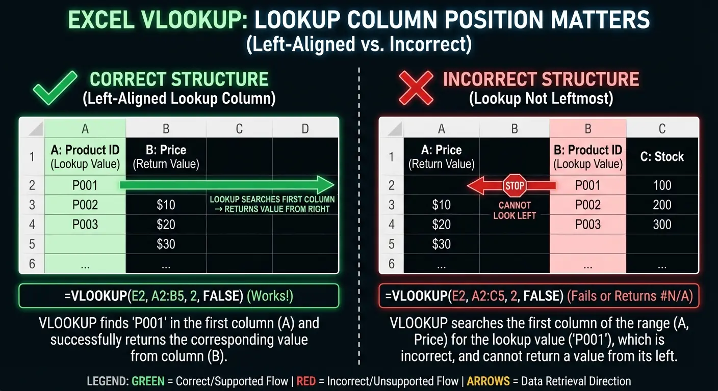
VLOOKUP only searches the leftmost column of your range and returns values to the right. This isn’t a bug. It’s how the function was built.

You need to structure your tables with the lookup column (the one containing your search values) positioned to the left of any columns you want to retrieve. If you’re trying to look up employee names and return their ID numbers, but the ID column is to the left of the name column, VLOOKUP can’t help you.

Restructure your table or use a different function.

This limitation forces you to think deliberately about table design. Your lookup column (customer ID, product SKU, employee number) should be the leftmost column because it’s the unique identifier for each row. Data you want to retrieve (customer name, product price, employee department) belongs to the right. This structure makes your spreadsheets more logical and easier for others to understand.

Formatting Consistency Isn’t Optional

Excel treats “100” (as a number) and “100” (as text) as completely different values, even though they look identical to you.

This formatting mismatch is responsible for more failed lookups than almost any other issue.

A friend at a mid-size manufacturer imports vendor data from their ERP every Monday. Vendor IDs come in as text: “V-2045”. Their Excel master list stores the same IDs as numbers with custom formatting. To the eye? Identical. To VLOOKUP? Completely different. She spent six weeks manually reconciling invoices before someone caught it. The fix took 90 seconds with a VALUE() function.

Your lookup value and the values in your search column must have identical formatting. Number vs. text, leading/trailing spaces, capitalization. All of it matters.

Use ISTEXT and ISNUMBER functions to check data types. Use TRIM to eliminate hidden spaces. And when you copy data from other sources (websites, PDFs, other spreadsheets), assume it’s introducing formatting inconsistencies until proven otherwise.

Duplicates Will Sabotage You Silently

VLOOKUP returns the first match it finds and stops searching.

If you have duplicate values in your lookup column, you’ll only ever retrieve data associated with the first occurrence. The other duplicates might as well not exist. This behavior causes subtle errors that are hard to catch because the formula technically works. It’s just returning the wrong data.

Duplicates in your lookup column mean your data’s broken. Period.

Sometimes duplicates indicate data quality issues that need fixing (multiple entries for the same customer). Fix them. Other times they’re legitimate (multiple transactions for the same product), which means VLOOKUP isn’t the right tool and you need SUMIF, COUNTIF, or a pivot table instead.

When comparing datasets to identify missing records, VLOOKUP’s ability to return #N/A values for unmatched records makes it a cornerstone function for many Excel applications (TechRepublic). This error-returning behavior becomes powerful for data reconciliation. But when duplicate lookup values exist, VLOOKUP’s limitation of returning only the first match means you’re working with incomplete information without realizing it.

Writing VLOOKUP Formulas (The Right Way)

Now that your data structure is solid, you’re ready to write the formula.

The syntax: =VLOOKUP(lookup_value, table_array, col_index_num, [range_lookup])

Microsoft Excel’s VLOOKUP function performs a vertical search from top to bottom for a value in the first column, then returns a result from the matching row (Windows Central). The function works by starting with information you know (the lookup value) and searching right to find information you don’t know (the return value).

Here’s how to build it parameter by parameter:

VLOOKUP Formula Construction:

=VLOOKUP(
    [Cell containing the value you're searching for],
    [Range containing both the search column and return column],
    [Number of the column you want to return],
    FALSE
)

Real example:

=VLOOKUP(A2, ProductTable, 3, FALSE)

What each part means:

• A2: The product ID I’m searching for

• ProductTable: Named range containing product IDs in column 1, descriptions in column 2, prices in column 3

• 3: I want the price, which is the 3rd column in my range

• FALSE: I need an exact match for this product ID

Selecting Ranges That Won’t Break Tomorrow

When you define your table_array parameter, don’t select exactly the range you need right now.

Your data will grow. If your VLOOKUP references a fixed range (like B2:D50), it stops working the moment you add row 51. You have two better options: use an entire column reference (like B:D) so the formula automatically includes new rows, or convert your data to an Excel Table (Insert > Table) and reference the table name.

Tables are better.

They expand automatically when you add rows and make your formulas more readable. Instead of =VLOOKUP(A2,$B$2:$D$50,2,FALSE), you write =VL

They expand automatically when you add rows and make your formulas more readable. Instead of =VLOOKUP(A2,$B$2:$D$50,2,FALSE), you write =VLOOKUP(A2,PriceTable,2,FALSE), which is self-documenting and maintenance-free.

The entire column reference approach (B:D) works well for most situations, though it can slow down performance if you have other data below your table in those columns. Excel will search through thousands of empty rows looking for matches that don’t exist. Tables solve this elegantly by maintaining clear boundaries so Excel knows exactly where your data ends.

Column Index Numbers That Survive Changes

The col_index_num parameter tells Excel which column to return from your range. If you specify 3, you’re getting the third column of your selected range.

This works fine until someone inserts a new column in the middle of your table, shifting everything and breaking your formula.

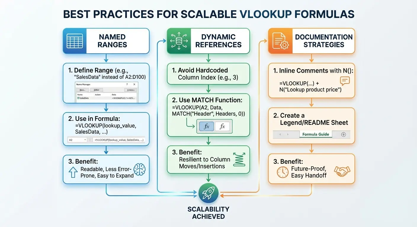
Instead of hardcoding column numbers, use the MATCH function to calculate them dynamically: =VLOOKUP(A2,B:E,MATCH(“Price”,B1:E1,0),FALSE)

This formula finds the “Price” header and returns data from that column regardless of where it moves. It’s more complex upfront but eliminates an entire category of maintenance problems. You’re building formulas that adapt to changes instead of breaking under them.

The Left-Side Thing Everyone Hates

We mentioned earlier that VLOOKUP only searches the leftmost column, but let’s dig deeper into what this means for your work.

This isn’t just a technical constraint to memorize. It’s a fundamental aspect of how VLOOKUP operates that should influence your entire approach to data organization. Many users spend hours trying to “fix” VLOOKUP when the real issue is they’re using the wrong tool for their table structure.

When the Limitation Actually Helps

The left-side constraint forces you to organize tables with a clear primary key on the left, which is good database design.

If you’re constantly fighting the left-side limitation, it might signal that your data isn’t organized optimally. Before you abandon VLOOKUP, consider whether restructuring your table would improve more than just your formulas. Better data architecture benefits every aspect of your spreadsheet, not just lookups.

When You Need to Look Left

Sometimes you genuinely need to return values from columns to the left of your search column, and VLOOKUP simply can’t do it.

Your options: INDEX MATCH (which can look in any direction), XLOOKUP (if you have Microsoft 365), or restructuring your table.

INDEX MATCH uses two functions together: MATCH finds the row position of your lookup value, and INDEX returns the value from that row in whatever column you specify. The syntax is less intuitive: =INDEX(return_column, MATCH(lookup_value, search_column, 0))

But it’s more flexible and doesn’t have the left-side limitation. You’ll need to decide whether learning a new function is worth the flexibility, or whether rearranging your columns is simpler for your specific situation.

Exact vs. Approximate Match (Get This Wrong and You’re Screwed)

The fourth parameter in VLOOKUP (range_lookup) is optional, which is dangerous because the default behavior causes massive problems if you don’t understand it.

When you omit this parameter or set it to TRUE, VLOOKUP uses approximate match mode, which finds the closest value that’s less than or equal to your lookup value. This is useful in specific scenarios (tax brackets, shipping rates, grade cutoffs) but catastrophic in most situations.

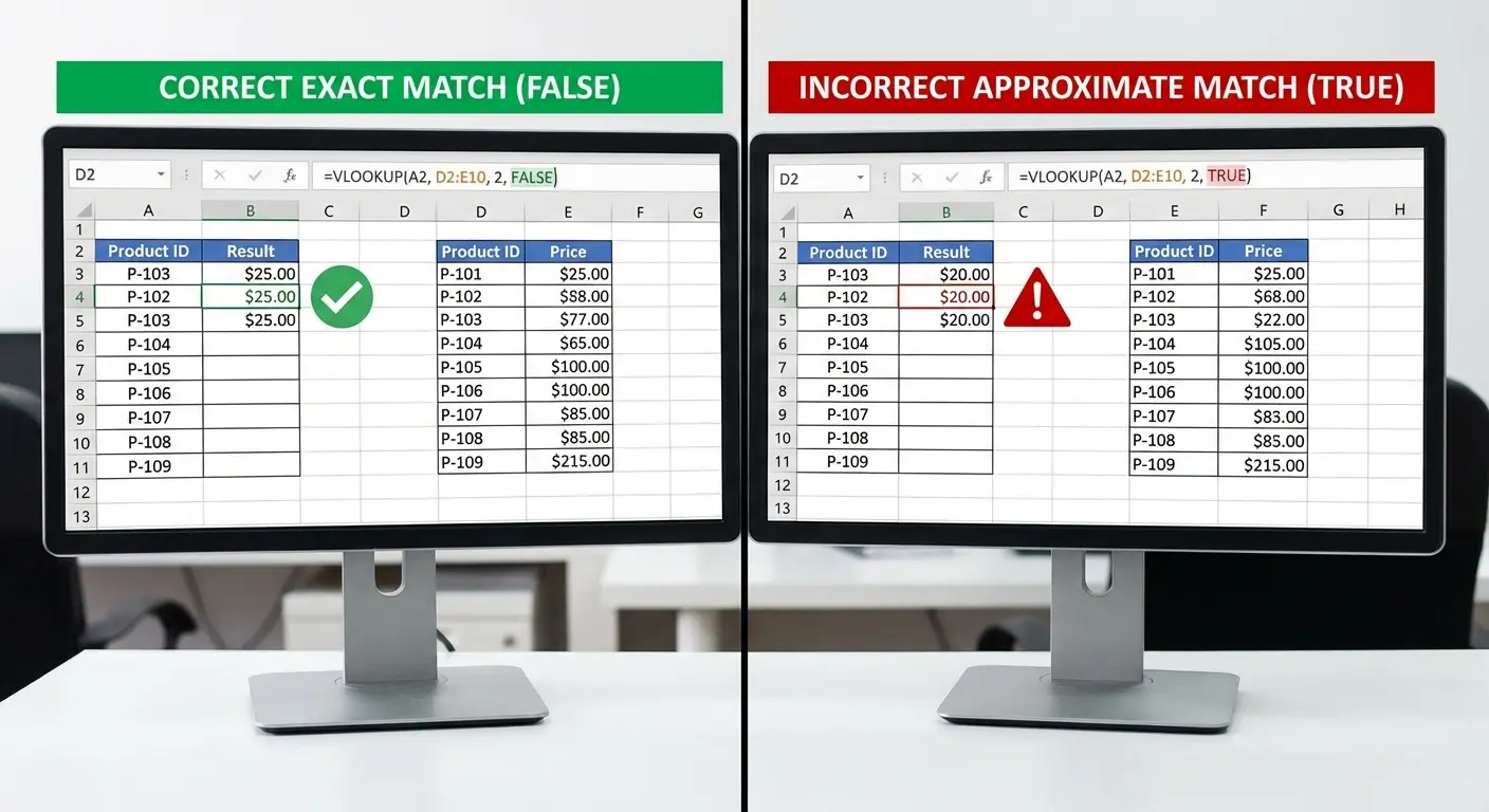
When you set it to FALSE, you get exact match mode, which only returns data for perfect matches.

Most of your lookups should use FALSE.

Match Mode	When to Use	What Happens on No Match	Risk Level
FALSE (Exact)	Looking up specific records (customer IDs, product SKUs, invoice numbers)	Returns #N/A error	Low (errors are visible)
TRUE (Approximate)	Range-based categorization (tax brackets, shipping tiers, grade scales)	Returns closest lower value	High (wrong data looks correct)
Omitted (defaults to TRUE)	Never intentionally omit	Returns closest lower value	Extreme (you didn’t intend this)

Why FALSE Should Be Your Default

Exact match mode (FALSE) does exactly what most people expect: it finds your lookup value or returns an error. You’re looking for customer ID 12345, and Excel either finds that exact ID or tells you it doesn’t exist.

This behavior is predictable and safe.

Approximate match mode (TRUE or omitted) does something completely different: it finds the largest value that’s less than or equal to your lookup value. If you’re looking for customer ID 12345 and it doesn’t exist, Excel might return data for customer ID 12340 instead. You won’t get an error. You’ll get wrong data that looks plausible, which is far more dangerous.

Always use FALSE unless you have a specific reason for approximate matching and your data is sorted correctly to support it.

The difference is so critical that experienced Excel users have developed a default practice: when the TRUE option is used for approximate matching, the first column often needs to be sorted, and failure to do so may cause unexpected results (Windows Central). This sorting requirement catches users off guard because VLOOKUP doesn’t warn you when your data isn’t sorted. It just returns incorrect values silently.

The safest approach is to always specify FALSE explicitly and only use TRUE when you’ve deliberately structured your data for range-based lookups.

The Rare Cases Where Approximate Match Makes Sense

Approximate match mode exists for situations where you need to categorize values into ranges.

You’re calculating shipping costs based on weight: 0-5 lbs costs $5, 5-10 lbs costs $8, 10+ lbs costs $12. You set up a table with the lower bounds (0, 5, 10) and corresponding costs, then use VLOOKUP with TRUE to find which bracket your package falls into. A 7 lb package matches to the 5 lb row and returns $8.

This works because your table is sorted in ascending order (required for approximate match) and you want range-based categorization.

But these use cases are uncommon. Most business lookups involve finding specific records (invoices, employees, products) where approximate matching produces incorrect results.

Error Handling That Actually Works

Every VLOOKUP will eventually fail to find a match.

Maybe someone deleted a record, misspelled an entry, or you’re looking up data that doesn’t exist yet. When VLOOKUP can’t find a match, it returns #N/A, which breaks any formula referencing that cell and makes your spreadsheet look unprofessional.

You need error handling built into every VLOOKUP formula. Not added later when problems appear. Every single one.

IFERROR: The Quick Fix

The simplest error handling wraps your VLOOKUP in an IFERROR function: =IFERROR(VLOOKUP(A2,B:D,2,FALSE),”Not Found”)

If the lookup succeeds, you get your data. If it fails, you get “Not Found” instead of #N/A. This prevents cascading errors and makes your spreadsheet more user-friendly.

You can customize the error message to provide context: “No price available” or “Check customer ID” tells users more than a generic error.

The limitation is that IFERROR catches all errors, not just missing matches. If you have a formula error (wrong column index, invalid range), IFERROR hides it instead of alerting you. For most situations, this tradeoff is acceptable. You’re preventing 95% of lookup errors with a simple wrapper.

Smarter Error Messages

Sometimes you need more sophisticated error handling that distinguishes between different failure modes.

You can use ISNA to check specifically for lookup failures while letting other errors surface: =IF(ISNA(VLOOKUP(A2,B:D,2,FALSE)),”Not Found”,VLOOKUP(A2,B:D,2,FALSE))

This formula runs the lookup twice, which isn’t efficient but provides more precise error handling.

For complex spreadsheets, you might add conditional formatting that highlights cells with missing lookups, or use data validation to prevent users from entering lookup values that don’t exist in your reference table. The sophistication you need depends on who’s using your spreadsheet and how critical accuracy is.

When VLOOKUP Becomes the Wrong Tool

VLOOKUP works beautifully for small to medium datasets with straightforward lookup requirements, but it has performance and functionality limitations that become problems as your needs grow.

You might not notice when you cross the threshold from “VLOOKUP is perfect for this” to “VLOOKUP is holding me back,” but there are clear signals.

Performance You Can’t Ignore

VLOOKUP searches sequentially from top to bottom, which means lookup speed degrades as your dataset grows.

With a few hundred rows, you won’t notice. With tens of thousands of rows and dozens of VLOOKUP formulas, your spreadsheet becomes sluggish. Every time you edit a cell, Excel recalculates all your formulas, and those VLOOKUP operations add up. You’ll notice longer save times, delayed responses when entering data, and general frustration.

INDEX MATCH performs better with large datasets because Excel can optimize the search process differently. If you’re experiencing performance issues and your spreadsheet contains multiple VLOOKUP formulas referencing large ranges, that’s your bottleneck.

Converting to INDEX MATCH or XLOOKUP often provides immediate performance improvements without changing your data structure.

Multiple Criteria Lookups Require Ugly Workarounds

VLOOKUP only searches one column, which creates problems when you need to match multiple criteria.

You want to find the price for Product X in Region Y during Quarter Z, but VLOOKUP can’t search three columns simultaneously. The workaround involves creating a helper column that concatenates your criteria (ProductXRegionYQuarterZ), then looking up that combined value.

This works but clutters your spreadsheet with artificial columns that exist only to make your formulas possible. It’s also fragile because anyone who doesn’t understand your system might delete the helper column and break everything.

Modern alternatives handle multiple criteria natively without helper columns. If you’re maintaining concatenated lookup columns, you’re working too hard.

The Maintenance Burden

VLOOKUP formulas require ongoing maintenance that compounds as your spreadsheet grows.

Column index numbers need updating when table structures change. Range references break when you reorganize worksheets. Hardcoded values become incorrect when your business logic evolves. Each individual maintenance task is small, but across dozens of formulas in multiple spreadsheets, the cumulative burden becomes significant.

You spend time fixing formulas instead of analyzing data.

Teams develop informal rules about “don’t touch column D” or “always insert columns on the right” to avoid breaking lookups. These workarounds signal that your formula strategy needs rethinking. Better tools exist that reduce maintenance overhead and make your spreadsheets more resilient to changes.

Building Formulas That Won’t Break Next Month

Write formulas that survive growth, changes, and collaboration.

This is about specific techniques that make your formulas more robust: using named ranges for readability, incorporating dynamic references that adapt to new data, documenting your logic for future users, and structuring your spreadsheets so formulas can be copied without breaking.

Think beyond “does this formula work right now?” and ask “will this formula still work in six months when we have twice as much data and three new team members using this spreadsheet?”

Named Ranges Make Everything Better

Instead of referencing $B$2:$D$100 in your formulas, name that range “PriceTable” and reference it by name.

Your formula becomes =VLOOKUP(A2,PriceTable,2,FALSE), which is self-documenting and easier to audit. Named ranges also provide a single point of maintenance. If your price table expands or moves, you update the named range definition once instead of editing every formula that references it.

Creating named ranges takes an extra minute upfront but saves hours over the life of your spreadsheet.

Go to Formulas > Name Manager to create and manage named ranges. Use descriptive names that indicate what the range contains (CustomerData, ProductCatalog, ShippingRates) rather than generic names (Table1, Range2).

Documentation Helps

Six months from now, you won’t remember why you structured a formula a certain way. Your colleague who inherits your spreadsheet definitely won’t know.

Add brief comments to complex formulas explaining the logic: “Looks up product price from master catalog, returns ‘Discontinued’ if product not found.”

Excel’s comment feature (Review > New Comment) lets you attach notes to specific cells. For particularly complex spreadsheets, create a dedicated documentation worksheet that explains your table structures, formula logic, and any assumptions or limitations.

This feels like busywork when you’re building the spreadsheet, but it’s invaluable later. Good documentation is the difference between a spreadsheet that others can maintain and one that becomes abandonware the moment you leave the project.

Test Against Edge Cases

Your VLOOKUP might work perfectly with your current data but fail when someone enters something unexpected.

Test your formulas against edge cases before deploying them: What happens if the lookup value is blank? What if someone enters text where you expect numbers? What if the reference table is empty? What if there are duplicate matches?

Create a test worksheet with problematic scenarios and verify your formulas handle them gracefully. This proactive testing catches problems before they reach users and helps you identify where you need additional error handling or data validation.

It’s also useful documentation because your test cases show others what scenarios you’ve accounted for.

Moving Beyond VLOOKUP Without Breaking Everything

You’ve recognized that VLOOKUP has limitations, and you’re ready to explore alternatives. But you have existing spreadsheets with dozens of VLOOKUP formulas that people depend on.

You can’t just rip everything out and rebuild.

Here’s a practical transition strategy that lets you adopt better tools gradually without disrupting your workflow.

Understanding Your Options

INDEX MATCH is the most powerful alternative available in all Excel versions.

It combines two functions: MATCH finds the position of your lookup value, and INDEX returns the value at that position from your chosen column. The syntax is =INDEX(return_range, MATCH(lookup_value, search_range, 0))

It can look left, doesn’t require column index numbers, and performs better with large datasets.

XLOOKUP is newer (Microsoft 365 only) and simplifies the syntax: =XLOOKUP(lookup_value, search_range, return_range)

It includes built-in error handling, can search from bottom to top, and handles multiple criteria more elegantly. If you have access to XLOOKUP, it’s generally the best choice for new formulas. If you’re on an older Excel version, INDEX MATCH provides similar capabilities with slightly more complex syntax.

Converting Existing Formulas

Don’t convert all your VLOOKUP formulas at once.

Start with the ones causing problems: formulas that break frequently, perform slowly, or require constant maintenance. Create a new column next to your existing VLOOKUP results and write the alternative formula there. Compare the results cell by cell to ensure they match.

This parallel testing catches conversion errors before you delete your working formulas.

Once you’ve verified the new formula works correctly, you can replace the old one. Document what you changed and why, especially if others use the spreadsheet. For critical spreadsheets, keep a backup with the original VLOOKUP formulas until you’re confident the new approach is stable.

Training Your Team

If you’re the only person using a spreadsheet, you can adopt new functions freely. But shared spreadsheets require team alignment.

Your colleagues need to understand the new formulas well enough to troubleshoot basic issues and avoid breaking them through well-intentioned edits.

Create simple documentation that explains the new formula structure with examples. Focus on the practical differences they’ll notice rather than technical details: “This new formula can look up values in any column, not just the first one” is more useful than a deep dive into function syntax.

Consider hosting a brief training session where you walk through a few examples. The goal isn’t making everyone an expert. It’s building enough familiarity that the new formulas don’t feel intimidating or mysterious.

When to Stick With VLOOKUP

VLOOKUP isn’t obsolete, and you don’t need to eliminate it from every spreadsheet.

For simple lookups in small datasets where your table structure is stable, VLOOKUP remains perfectly adequate. It’s also more widely understood than alternatives, which matters if your spreadsheets are used by people with varying Excel skills.

The transition to other functions should be driven by specific problems or limitations, not a desire to use the newest tools. If your VLOOKUP formulas are working reliably and efficiently, leave them alone.

Focus your energy on situations where VLOOKUP genuinely holds you back.

Final Thoughts

Three things matter: clean data, exact match mode, and knowing when you’ve outgrown VLOOKUP.

Everything else is just details.

VLOOKUP problems are almost never formula problems. They’re data architecture problems, planning problems, and scalability problems that manifest as formula errors. When you shift your focus from “how do I write this formula?” to “how do I structure my data so lookups are reliable and maintainable?”, everything changes.

You spend less time troubleshooting and more time extracting value from your data. You build spreadsheets that others can understand and maintain. You recognize earlier when you’ve outgrown a tool and need something more powerful.

Start with proper data structure. Build formulas that account for failure modes. Always prioritize maintainability over cleverness.

Now go fix your spreadsheets.